Prediction intervals for time series
What it is all about
Most of the practical implementations of predictive scenarios heavily focus on delivering single-point based predictions. What does that mean? That means, when getting a prediction, you get one predicted sample per timestamp. As a result, you do not get any information on how “certain” or “uncertain” the model is when predicting the future data points. As an enduser relying on the predicted data points, for example, in a financial forecasting scenario in a business department, knowing nothing about the “certainty” of the model can lead to huge problems. When basing decisions on the predicted data points, knowing when to trust the predictions and when to be careful is crucial for enduser adoption of the implemented machine learning forecast.
Let’s get the idea behind having prediction intervals instead of single-point predictions using an example. The example dataset is about electricity demand forecasting and can be found here (https://raw.githubusercontent.com/scikit-learn-contrib/MAPIE/master/examples/data/demand_temperature.csv).
The first figure shows single-point predictions made with a random forest regressor.
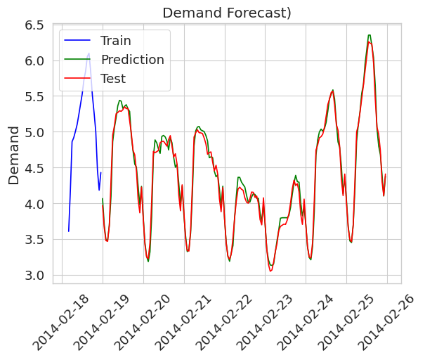
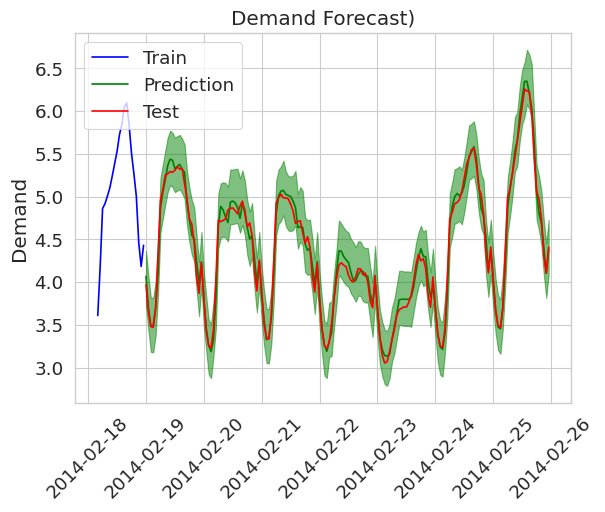
The single point predictions do not give any information to the user about model uncertainty, whereas a prediction with prediction intervals does so. The following figure shows the same setting but with prediction intervals (created using the EnbPI algorithm).
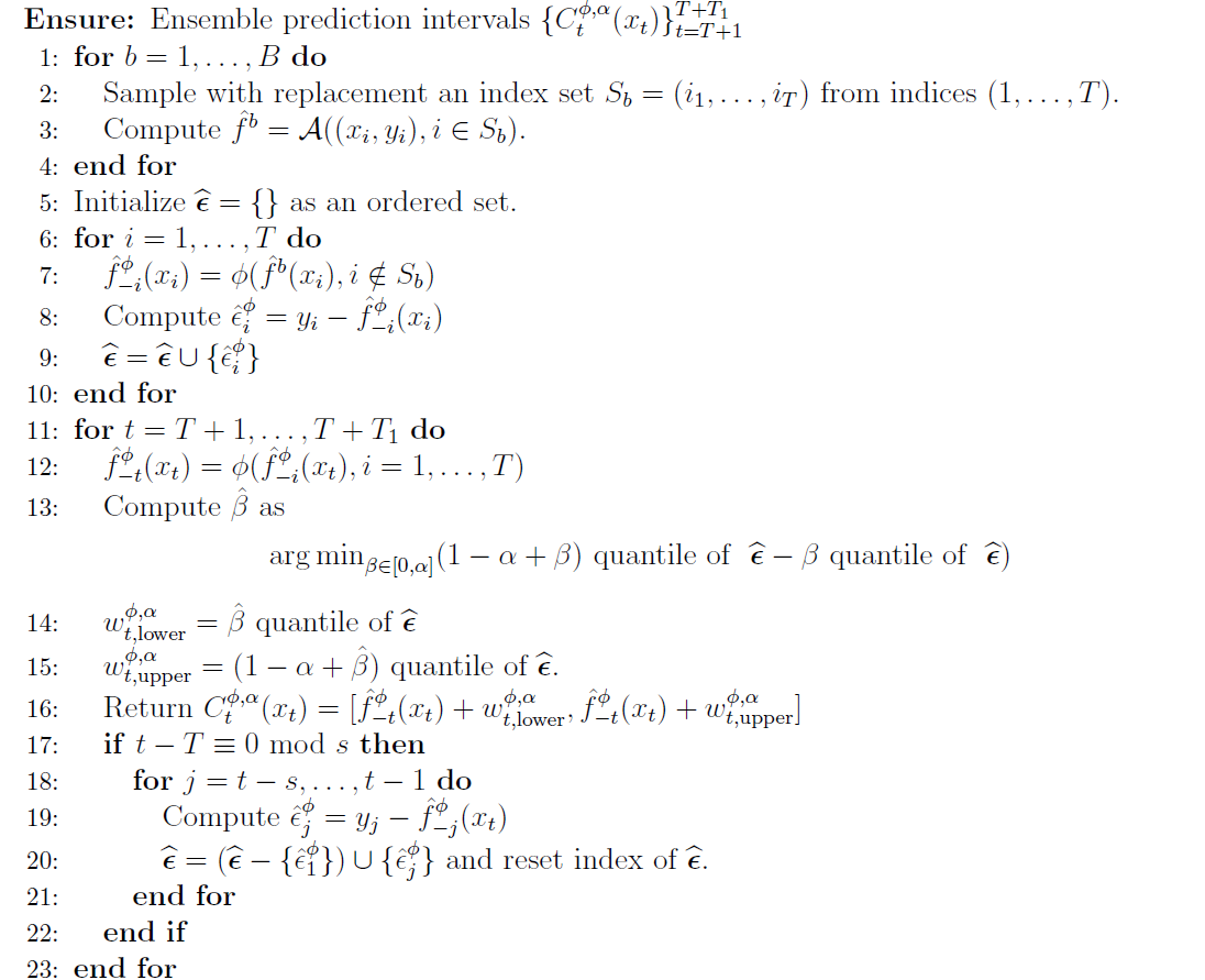
A milestone for prediction intervals for time series data, is the EnbPI algorithm, which I am going to explain in the following. The algorithm is taken from the original paper. The comments are based on my personal understanding and intuition and on remarks the authors give in their respecitve paper.
The idea in a nutshell
Roughly speaking (very rough), very simplified:
To get a prediction interval $C$ instead of a single point prediction we need to somehow get the uncertainity the model produces for the prediction. The algorithm does this, by using the errors the estimated model $\hat{f}$ produces when predicting data from the training set (see the residuals $\epsilon$ in the algorithm). This can be done, as we know the target values $y_i$ for each training sample.. To produce the minimum, maximum and mean of the prediction interval the algorithm not only uses one predictor $\hat{f}$, but an ensemble that is trained in an efficient and intelligent way (on different subsets of the data, see the sampling procedure in the data). The mean of the interval is computed using the mean predictions (or median, … therefore generally denoted as $\phi$ in the algorithm below) of these ensembles, and the minimum and maximum bounds are computed using the past errors of the ensemble models.
Input to the conformal prediction algorithm
- Training data ${(x_i, y_i)}_{i=1}^T$
- Our prediction (forecasting) algorithm $A$
- The significance level $\alpha$ for the coverage we desire
- An aggregation function $\phi$. I will replace the $\phi$ symbol in the following using the abbreviation $agg$ for simplicity. The aggregation function is simply a function that aggregates multiple scalar values into one, such as, the mean, the median, or something else. Usually, we just take the mean
- Another hyperparameter for the conformal prediction algorithm is the batch size $s$, that we use to split our training data into subsets.
- Where would we be without some test data (or new data in a productive setting) that was NOT used for training our prediction algorithm. ${(x_t, y_t)}_{t=T+1}^{T+T_1}$. Timestep $t$ is not part of the timesteps in our training data $T$. Of course, we do not immediately know $y_t$, but we will use the target value $y_t$ of our new data point $t$ for creating future intervals. Any why is that you might think: We do not know $y_t$ of a new sample immediately, because this is what the whole prediction is about :) We want to predict this target value.
So we have everything in place, the data we need, the prediction algorithm we selected, the hyperparameter values for the conformal prediction algorithm and some new data that we want to compute prediction intervals for.
Other symbols / hyperparameters
-
$s$ is the number of future steps the predictor predicts into the future in one inference run.
-
$S$ simply denotes an index $S$et
-
$\hat{f}_{-i}$ denotes that the estimated predictor $\hat{f}$ is estimated without (i.e. the minus sign) the data sample with index $i$
-
To denote the training subset the estimated predictor $\hat{f}$ was trained on, we add the number $b$ of the subset $S_b$ to the estimator $\hat{f}^b$. For the estimators that are based on the aggregation of other estimators we add the aggregation function $\phi$ as the superscript $\hat{f}^\phi$.
Full Algorithm
With the input in place, we will walk through the full algorithm and also turn it into a simple python implementation to see how the individual steps play out.
Part 1: Using the training data to gather information about the predictor
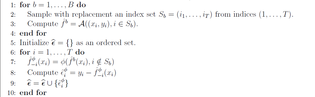
As we aim to train multiple models of our predictive estimator, we need to have subsets of our training data to train them. Training the models on the same data would make no sense of course.
Randomly sampling data from the training time series would completely violate the correlation of the time series data. Therefore, the authors use block boostrapping: the method simply divides the time series into subsequences of a certain size. Then, not individual data points are sampled to construct a new time series, but the blocks are sampled.
In fact, one can compare the first block (show above) of the algorithm to the “fit” training procedure in machine learning algorithms. The following python code, shows my implementation of this pseudo-code block in a python “fit” function. You can correlate the python code with the pseudo-code from the paper by having a look at the comments in the code :) (Note that the code is not optimized and does not account for input problems, etc.!)
    def fit(self, x_train, y_train,  block_size, aggregation_function = np.mean, n_batches = 10, batch_sequence_length = 6):
        """Fit the model to the training data.

            Args:
                x_train (array-like): The input training data.
                y_train (array-like): The target training data.
                block_size (int): The number of consecutive data points in each block.
                aggregation_function (function, optional): The function used to aggregate the predictions of the models trained on different batches. Defaults to np.mean.
                n_batches (int, optional): The number of batches to sample. Defaults to 10.
                batch_sequence_length (int, optional): The length of the batch sequence. Defaults to 6.
        """
        # Prepare block sampling
        # Create blocks of consecutive data points of the time series
        block_size = 3 # number of consecutive data points in each block

        train_indices = np.arange(1, len(x_train)) # indices of the training data
        train_indices_blocks = np.array_split(train_indices, block_size) # split the indices into blocks
        block_indices = np.arange(len(train_indices_blocks)) # indices of the blocks

        # Start of sampling procedure
        number_of_blocks_to_sample = math.ceil(batch_sequence_length / block_size)


        self.f_b_dict = {} # store all f_b models for each batch in a dictionary
        self.batches = {} # store all batches in a dictionary
        # The following procedure corresponds to line 1 to 4 in the algorithm

        for b in range(1, n_batches):
            batch_x = []
            batch_y = []
            for n in range(number_of_blocks_to_sample):
                block_index = np.random.choice(block_indices)
                batch_x.extend(x_train[train_indices_blocks[block_index]])
                batch_y.extend(y_train[train_indices_blocks[block_index]])

            self.batches[b] = {"x": batch_x, "y": batch_y, "indices" : train_indices_blocks[block_index]}

            print(f"X: {batch_x}")
            print(f"Y: {batch_y}")
            print("---------------------------------------")

            # Train the model on the batch
            f_b = self._estimator.fit(batch_x, batch_y)
            self.f_b_dict[b] = f_b # save the model f_b for each batch

        # Line 5: Initialize error (residual) list
        self.residual_e_list = []

        self.f_phi_minus_i_dict = {} # store all f_phi_minus_i models for each batch in a dictionary
        # Line 6: iterate over all training data points
        for i in range(1, len(x_train)): # len(x_train) corresponds to T in the pseudo code
            # Get all batches that do not contain the current data point i
            # use the respective model to predict the output
            # collect the results of all models that are trained on data that do not contain i
            # and apply the aggregation function (mean in this case) to the data

            f_b_minus_i_list = []
            for b in self.batches.keys():
                if i not in self.batches[b]["indices"]:
                    f_b_minus_i_list.append(self.f_b_dict[b])

            # Line 7: Compute the aggregated function
            f_phi_minus_i = lambda x: aggregation_function([f_b_minus_i.predict(x) for f_b_minus_i in f_b_minus_i_list])
            self.f_phi_minus_i_dict[i] = f_phi_minus_i

            # Line 8: Calculate the residual for data point i
            e_phi_i = y_train[i] - f_phi_minus_i(x_train[i].reshape(1, -1))

            # Line 9: add to residual list
            self.residual_e_list.append(e_phi_i)

            self._isfit = True
Part 2: Creating intervals on new data using the past performance of the predictors
When computing the prediction intervals based on the past residuals $\hat{e}$ there are multiple ways to do this. We could use all $\hat{e^\phi_i}$ values we have. By doing so, we would incorporate all the uncertainty and potential model errors we can in our prediction interval. But the interval would be huge. This is not very useful, we want intervals that satisfy our alpha level (our specified coverage hyperparameter = roughly said, the probability the final interval will contain the true prediction, given the model).
Thus, we estimate a threshold probability ($\beta$) to get a prediction interval that is just large enough and as narrow as possible to guarantee, given the mode, the coverage we want.
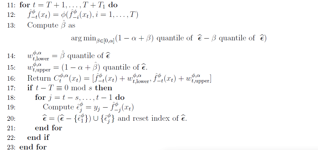
Analogous to the first block of the algorithm, I have created a python function “predict” for creating the intervals on new data points.
    def predict(self, x_test, alpha = 0.05):
        """Predict with the conformal prediction intervals

        Args:
            x_test (array-like): The input data.
            alpha (float, optional): The significance level for the prediction intervals. Defaults to 0.05.

        Returns:
            array-like: The predicted values.
        """
        if not self._isfit:
            raise RuntimeError("You must fit the algorithm before predicting data!")

        # Line 10: Calculate the prediction intervals
        # Compute the prediction intervals for each future (test) data point
        # Line 11: iterate over all future (test) data points
        prediction_intervals = []
        self.f_phi_minus_t_dict = {}

        for t in range(len(x_test)):

            # Line 12: compute the aggregated function of the prediction for t of all f_phi_not_i models
            f_phi_minus_t = lambda x_t: self._aggregation_function([self.f_phi_minus_i_dict[k](x_t) for k in self.f_phi_minus_i_dict.keys()])

            self.f_phi_minus_t_dict[t] = f_phi_minus_t
            # Line 13: compute beta to get the prediction interval that is as narrow as possible
            # we do the argmin procedure from the paper by simply creating a list of possible beta values between 0 and alpha
            # and pick the minimum according to the equation in the pseudo code in line 13
            # there would be a more efficient way to do this, but this is easier to understand
            beta_candidate_list = np.linspace(0, alpha, 100) # 100 values between 0 and alpha as candidates for beta
            get_beta_quantiles = lambda beta: np.quantile(self.residual_e_list, 1- alpha - beta) - np.quantile(self.residual_e_list, beta) #function to cmpute the quantiles according to the equation in line 13
            beta_quantiles = [get_beta_quantiles(beta) for beta in beta_candidate_list] #compute potential quantiles using the beta candindates
            beta = beta_candidate_list[np.argmin(beta_quantiles)] #get the narrowst quantile (argmin) that fullfills the coverage guarantee, and get the corresponding beta value

            # Line 14: compute the lower bound of the prediction interval using beta
            omega_phi_alpha_t_lower = np.quantile(self.residual_e_list, beta)

            # Line 15: compute the upper bound of the prediction interval using beta
            omega_phi_alpha_t_upper = np.quantile(self.residual_e_list, 1- alpha - beta)

            # Line 16. construct final prediction interval
            # do the prediction using the aggregated function f_phi_minus_t first, as this is the center of the prediction interval
            y_t_predicted = f_phi_minus_t(x_test[t].reshape(1, -1))
            c_phi_alpha = [y_t_predicted - omega_phi_alpha_t_lower, y_t_predicted + omega_phi_alpha_t_upper]

            prediction_intervals.append(c_phi_alpha)

            # Line 17 to line 22: Stopping criterion if all future datapoints have been iterated over
            # Here we update the residual list, this is ommited here as we do not have the true y_t values for now
            # for this purpose we have the predict_with_update function

        return prediction_intervals
The full class, contains some initialization besides the “fit” and the “predict” function:
def __init__(self, estimator, aggregation_function = np.mean):
    self._isfit = False
    self._estimator = estimator
    self.residual_e_list = None
    self._aggregation_function = aggregation_function
Professional Implementation of EnbPI
For real use cases, please use the implementation of the algorithm in the MAPIE library for conformal predictions.
Doing so, results in the prediction interval plot in the introductionary section of this blog post :)
You can find a full working example in the MAPIE documentation here (https://mapie.readthedocs.io/en/latest/examples_regression/2-advanced-analysis/plot_timeseries_enbpi.html ) so I refrain from copy - pasting it for my blog post :)