Accumulative local effects
ALE is a model-agnostic method for explaining the influence of features on predictions. It focuses on the global influence of a particular feature (or feature combination) on predictions, rather than explaining individual predictions. ALE overcomes some of the issues faced by Partial Dependence Plots (PDP), such as dealing with correlations between features.
Computation
At its core, ALE involves the following steps:
- Select a feature and consider each value that the feature can take.
- Create a small interval around each individual value and slightly vary the feature value within that interval.
- Observe how the predictions change as the feature values are wiggled.
- he computation of ALE involves sums instead of integrals, as integration over features may not be efficient.
To compute the ALE, we determine the difference in predictions for individual samples. By varying the feature of interest within a defined interval, we observe how the predictions change locally around that feature value. This is done by creating a neighborhood around a specific feature value, identifying the data instances within that window, and repeating the computation to observe the predicted outcomes.
By averaging the effects over the samples within the neighborhood, we obtain the ALE estimate. In contrast to Partial Dependence Plots (PDP), ALE plots only average over instances that lie within a small window around each feature value, instead of forcing all instances to have a fixed value for the feature
Molnar describes this in his book as follows: “Let me show you how the model predictions change in a small”window” of the feature around v for data instances in that window.”
The estimate of the ALE using the following notation:
- feature number j
- input data x
- sample number i
- input data sample $x^{(i)}$
- feature j of input data sample $x_j^{(i)}$
- k is one value feature j can have (we assume a grid of values k to discretize continous ones)
- neighborhood (interval) for value k of feature j: $N_j(k)$
- a sample $x_j^{(i)}$ can be within a neighborhood $N_j(k)$ if its value for feature j is close to k
The ALE computes the difference in predictions for certain neighborhoods of a feature j. Each feature j hast multiple values k it can assume. So we get one “difference” in prediction per value k. Each neighborhood can contain a different number of samples. Thus, we average over these samples, i.e. we divide by the number of samples $x_j^{(i)}$ in a certain neighorhood
The formula for computing the ALE (for estimating it using sums):
\[\hat{\widetilde{f}}_{j, ALE}(x) = \sum_{k=1}^{k_j(x)} \frac{1}{n_j(k)} \sum_{i:x_j^{(i)} \in N_j(k)} \left[ \hat{f}(z_{k,j}, x^{(i)}_{ - j})- \hat{f}(z_{k-1,j}, x^{(i)}_{ - j}) \right]\]So we have some additional notation in here:
- $\hat{\widetilde{f}}_{j, ALE}(x)$ is our uncentered ALE estimated, based on the estimator $\hat{f}$
- $\hat{f}$ is our estimator, our machine learning model
- $\hat{f}_{j, ALE}(x)$ ist die estimated ALE value for feature j, using the input data x
- $k_j(x)$ is the last value k feature j can assume for data point x
- $n_j(k)$ is the number of data points $x_j^{(i)}$ in the Neighborhood $N_j(k)$
- $\sum_{i:x_j^{(i)} \in N_j(k)}$ sums over all data points in the neighborhood $N_j(k)$ for feature j
Now to the weird part at the heart of the equation:
- $z_{k,j}$ is a value from a grid $Z$ that we define to vary our feature j (the intervals we construct) We have this interval for each value $k$ the feature $j$ assumes. So we call this grid value $z_{k,j}$
- $x^{(i)}_{ - j}$ is just the datapoint $x^{(i)}$ without the feature $j$ (notated by using $-j$) We just remove the “column” $j$ from the feature vector $x^{(i)}$
- $x^{(i)}_{ - j}$ has one column removed. The column $j$. So we can not input it into our estimator. We need to add the “column” $j$ again. But we want to wiggle around the value $k$ of column $j$ a little bit to get the difference in prediction our wiggling causes (wiggling = slightly editing the value $k$ = a small interval around $k$ = our grid values from $Z$).
Thus we compute: $\hat{f}(z_{k,j}, x^{(i)}{ - j})$ And with the previous grid value $z{k-1,j}$ we get $\hat{f}(z_{k-1,j}, x^{(i)}_{ - j})$ respectively
How does this grid look like? That is one crucial part when implementing ALE. So let’s say for a numerical featuere that assumes the values $[1,2,3]$ we define for each $k\in[1,2,3]$ the grid.
Then our grid can look like: $Z = [0.5,1.5,2.5,3.5]$
So for $k=1$ we have $z_{1,j} = 1.5$ and $z_{k-1,j} =z_{0,j} = 0.5$
or for $k=3$ we have $z_{3,j} = 3.5$ and $z_{3-1,j} =z_{2,j} = 2.5$
As you can see if we have $k$ values, we need $k+1$ values in the grid $Z$. We add a $k=0$ value, altough in our formula we sum over all $k$ starting at $k=1$.
We merge these values back into the original data point and obtain a perfectly fine, slightly tunes data point vector for sample $i$. We run the two tuned vectors we obtain per $k$ throug our model, compare the predictions, and go on :)
The construction of the grid depends on the type of variable (numerical, continuous, categorical), and it is an important implementation detail in ALE. We aim to distribute the number of data points within each neighborhood as equally as possible when designing the grid. One approach is to use quantiles (percentiles) of the feature column values, ensuring an equal number of data points in each interval.
After computing the uncentered ALE estimate $\hat{\widetilde{f}}_{j, ALE}(x)$, we center it, so that the mean effect is zero over the column.
\[\hat{f}_{j, ALE}(x) = \hat{\widetilde{f}}_{j, ALE}(x) - \frac{1}{n} \sum_{i=1}^n {\hat{\widetilde{f}}_{j, ALE}(x^{(i)}_j)}\]So, for the ALE of a feature, we take the individual ALE estimates and averages over all samples (i.e. indirectly over the possible values $j$ can have).
Now we have the centered ALE estimate (mean effect is zero): $\hat{f}_{j, ALE}(x) $
\[\hat{\widetilde{f}}_{j, ALE}(x^{(i)}_j) = \sum_{k=1}^{k_j(x^{(i)}_j)} \frac{1}{n_j(k)} \sum_{i:x_j^{(i)} \in N_j(k)} \left[ \hat{f}(z_{k,j}, x^{(i)}_{ - j})- \hat{f}(z_{k-1,j}, x^{(i)}_{ - j}) \right] = \frac{1}{n_j(k)} \sum_{i:x_j^{(i)} \in N_j(k)} \left[ \hat{f}(z_{k,j}, x^{(i)}_{ - j})- \hat{f}(z_{k-1,j}, x^{(i)}_{ - j}) \right]\]Example computation on bike rental dataset
Load the dataset first, and pre-process it, according to the procedure in the interpretable ml book
import data_preprocessing as dp
import warnings
warnings.filterwarnings("ignore")
data = dp.get_bike_data('data/bike_sharing/day.csv')
X = data.drop(["cnt"], axis=1)
Y = data["cnt"]
from sklearn.preprocessing import OrdinalEncoder
encoders = {}
# Encode all categorical variables
for col in X.columns:
    if X[col].dtype == 'category':
        if col == "season":
            order = ["spring", "summer", "fall", "winter"]
        elif col == "weathersit":
            order = ["GOOD", "MISTY", "RAIN/SNOW/STORM"]
        elif col == "mnth":
            order = ["jan", "feb", "mar", "apr", "may", "jun", "jul", "aug", "sep", "oct",
                     "nov", "dec"]
        elif col == "weekday":
            order  = ["sun", "mon", "tue", "wed", "thu", "fri", "sat"]
        else:
            order = []

        if len(order) > 0:
            # make elements in order uppercase
            encoder = OrdinalEncoder(categories=[[o.upper() for o in order]])
        else:
            encoder  = OrdinalEncoder()

        encoder = encoder.set_output(transform="pandas")
        X[col] = encoder.fit_transform(X[[col]])
        encoders[col] = encoder
We need to have an estimator, our predictor, that we can interpret. We will train a tree regressor model and see how the features influence the predictions using ALE.
from sklearn.tree import DecisionTreeRegressor
regressor = DecisionTreeRegressor(random_state=0)
regressor = regressor.fit(X, Y)
ALE for Continious Feature
We take the temperature feature as an example for a continious feature
Step by step we will compute the ALE
import numpy as np
def compute_ale(X, feature_name, z_j, return_individual_values=False):
    """_summary_

    Args:
        X (_type_): input data frame
        feature_name: name of the feature
        z_j (_type_): grid with the intervals
        return_individual_values (_type_): whether to return the individual values or not
    """
    feature_j = X[feature_name].values
    k = np.unique(feature_j) # our value vector k of the unique values in feature j

    feature_j_grid_cell = np.digitize(feature_j, z_j, right=False) # digitize returns the index of the bin that the feature value falls into

    # for each sample point, we have the bin it falls into
    # we start at z_j[1:], because the first element is not a bin we want datapoints to fall into
    # refer to the formula above for details
    sum_over_all_values_k = []

    # we have the different values k of the feature j
    # multiple values k can fall into the same bin
    # we average over all the k's that fall into the same bin
    # so first, for each k, we will find all the samples that fall into the same bin
    # then we can go over all the samples in that bin and compute the difference in prediction

    # for each sample point, we create one wiggled data point with the value of the bin, and one wiggled point with the value of the previous bin
    # for each bin, find all the value k's that fall into it

    for bin_idx, bin in enumerate(np.unique(feature_j_grid_cell)):
        samples_in_bin_indices = np.argwhere(feature_j_grid_cell[feature_j_grid_cell == bin]) # the samples within a bin, i.e. within the neighborhood of the bin
        if samples_in_bin_indices.size == 0:
            continue
        difference_in_prediction_inner_sum = []
        samples_in_neighborhood = X.iloc[samples_in_bin_indices.flatten()].copy()
        for index, sample in samples_in_neighborhood.iterrows():

            z_j_k = z_j[bin_idx] # first grid cell
            z_j_k_minus_1 = z_j[bin_idx-1] # previous grid cell

            x_i_z_j_k = sample.copy()
            x_i_z_j_k[feature_name] = z_j_k

            x_i_z_j_k_minus_1 = sample.copy()
            x_i_z_j_k_minus_1[feature_name] = z_j_k_minus_1

            # get the difference in prediction
            difference_in_prediction_for_x_i = regressor.predict(x_i_z_j_k.values.reshape(1, -1)) - regressor.predict(x_i_z_j_k_minus_1.values.reshape(1, -1))
            difference_in_prediction_inner_sum.append(difference_in_prediction_for_x_i)

        averaged_difference_in_prediction = np.sum(difference_in_prediction_inner_sum) * 1/len(  samples_in_neighborhood)


        sum_over_all_values_k.append(averaged_difference_in_prediction)

    ale_uncentered = np.sum(sum_over_all_values_k)
    ale_centered = ale_uncentered - 1/len(feature_j) * np.sum(sum_over_all_values_k)

    if return_individual_values:
        return ale_centered, sum_over_all_values_k
    else:
        return ale_centered
We also create one function to create the grid for continious columns
def create_grid_continious(feature_j, grid_size=10):
    k = np.unique(feature_j) # our value vector k of the unique values in feature j
    percentile_cut_offs = np.linspace(0, 100, grid_size) / 100 # number of percentile values to compute
    z_j = np.quantile(k, percentile_cut_offs) # compute the percentile values, k+1 values, as needed for the grid Z
    return z_j
z_j = create_grid_continious(X["temp"].values, grid_size=100)
ale_centered, sum_over_all_values_k = compute_ale(X, "temp", z_j, return_individual_values=True)
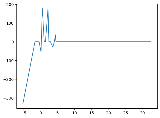
Plot the ALE
# plot the ALE
import matplotlib.pyplot as plt

# plot the ALE
plt.plot(z_j, sum_over_all_values_k)
plt.show()
Sources
Bike dataset pre-processing functions, similiar to the ones provided in R: https://github.com/christophM/interpretable-ml-book/blob/master/R/get-bike-sharing-dataset.R
Main source: https://christophm.github.io/interpretable-ml-book/ale.html