Exploring explainable boosting machines

To all those who love Star Wars :) (The others are free to ignore the following paragraph)

'Black-boxes are without alternative' is a lie. There is only ignorance.

Through linearity, I gain Interpretabilty.
Through trees, I gain Predictive Power.

Through Predictive Power, I gain Victory.

Through Victory, my chains are broken.

EBMs shall free me.

(and a pretty nerd, supported by chatGPT, I am)

Motivation

In real-world projects you often face the following decision: either you make a model interpretable or no one will use it to make decisions.

Linear models are an all-time favourite to machine learning practitioners because they are easy to interpret. They are often called “white-box” or glass-box models because the inner workings of the model can be understood by looking at the weights assigned to each feature. This makes it possible to evaluate the contribution of each feature to the overall prediction, both globally (across all data points) and locally (for individual data points).

However, linear models have limitations. They are not well-suited for handling interactions between features or non-linear relationships to the outcome variable. Imagine trying to predict housing prices using only two variables: square footage and number of bedrooms (example taken from ¹). With a linear model, you could easily capture the impact of each variable on the predicted price. But what if the number of bedrooms is more important for smaller houses, while square footage is more important for larger houses? A linear model would struggle to capture this kind of non-linear relationship.

This is where more complex models like neural networks come in. Neural networks are capable of capturing non-linear interactions between features, which makes them highly predictive. However, this comes at the cost of interpretability. It’s hard to know exactly how a neural network arrived at a particular prediction, which can be a problem when it comes to making important decisions based on the model’s output. In practice, this renders these black box models unusable for many real-world problems as machine learning models are (mostly) finally used by some human being that wants to know what is going on in the model.

To walk the line between interpretability and predictive power, machine learning practitioners have developed algorithms like (Generalized) Additive Models (GAMs) and Explainable Boosting Machines (EBMs). These models are capable of capturing non-linear relationships between features while also providing insights into how the model arrived at a particular prediction. By using models like these, decision-makers can have more confidence in the model’s output and use it to make more informed decisions.

One family of models that can be used in these scenarios is called General Additive Models (GAM), and in particular the Explainable Boosting Machine (EBM) model from this family, and we will get into the nitty-gritty details of these algorithms during the time we spend together in this blog post.

More than linear

Additive models extend mere linear models by replacing the scalar (“one-value”, “just a simple number”) weights $\beta_i$ with individual functions $f_i$ ².

This leads to more predictive power at the end. But how?

Take the simple linear model. Each weight in the model scales, for each individual data point, the value of the respective feature. So let’s say, our feature is called “daily_sales”. Then our weight $\beta_{daily_sales}$, is a single number, for all values our feature “daily_sales” can take. It does not care about the exact value “daily_sales” has. If our weight equals, for example, $\beta_{daily_sales}=10$ it will multiply our “daily_sales” value by 10, whether we sold $1$ unit or $1.000.000$ units on a particular day. The model does as it is told: it assumes a simple linear relationship for each feature with the target, so having this individual weight per feature is sufficient. You can think of it as the slope of the line relating the feature values to the outcome. In a simple, linear line (I know …) the slope is constant.

But this is not very expressive. When we have non-linear relationships, this leads to bad predictions. And our stakeholders won’t be happy and you will have a bad day presenting the results of your project.

Imagine, for each feature, instead of a fixed weight $\beta$, you could use an arbitrarily complex function. Then, the contribution of each feature to the prediction is still clear, as the function you choose just replaces the isolated, individual weight $\beta$ of an individual, isolated feature.

But you could, for example, multiply high “daily_sales” values with more weight than low ones, because they have more influence on the final outcome. In our secret, arbitrary function you assign a weight of $100$ to data points that include more than $1.000.000$ sold units in the feature “daily_sales”, while still using a $10$ multiplier weight for datapoints that have less than $1.000.000$ units sold. This is clearly non-linear, and will improve your predictions if the relationship to the oucome resembles this non-linearity.

Do you see where this is going?

So far, I have talked about regression tasks, but these models can be easiliy extended for classification by turning the predictions the model makes (i.e. some unconstrained number) into probabilities. These probabilities can then be turned into class values by applying a threshold to the probability. In the binary case, we just apply a function to the result of the additive general model, that turns the predictions into into probabilities for a certain class, i.e. values between 0 and 1 ². We can do so by applying the inverse logit function to our output. It maps our regression output to a range of values between 0 and 1 ².

Nice. But everything needs a name.

So we call this little piece that allows us to link our regression results to classes in a classification task, the (drums …. ) link function . ². Then we set, for example, a threhsold at $0.5$ to assign all instances that have a predicted probability above $0.5$ for class 1 to class 1. This is a rather straight forward and simple idea, the math of it is explained in more detail in the interpretability section at the end of this post, when we talk about how to interpret EBM outputs for classification tasks.

It is just a poem …

I could not resist to ask my favourite large-language mode to do my the favor of creating a small piece for this blog post:

In the forest of shallow trees,
A thin line stands tall and free,
Each one reaching for the light,
Capturing sun with all their might.

Together they create a sight,
A perfect union shining bright,
Their trunks and branches intertwined,
A symbol of nature's design.

In this place where shadows play,
And light and dark dance and sway,
The trees stand proud, their work well done,
A perfect line, a union one.

That’s all you need to know about explainable boosting machines. Somewhat. Maybe :) Or you read on an get to know some of the stuff this poem mentions.

Explainable Boosting Machines are not the only kind of Generalized Additive Model, and by far, not the first ones.

EBMs learn the individual functions for each feature $f_i$ by using techniques called gradient boosting and bagging. Behind the scenes, EBMs make use of a combination of a linear model and combination with decision tree algorithms ³. Let’s unravel the parts that make up EBMs step by step.

So, how does the boosting work in EBMs

Stripping the details of boosting techniques, what remains is that we have multiple algorithms (often of the same kind, such as decision trees) that are processing / and learning from the data in a sequential way. What this means is, we fit a first model and compute the error on the objective function with the training data. Then we fit a second model to reduce the error produced by the first model. And we fit a third model to reduce the error produced by the first two models, … and so on.

Think of the booster from Mario Kart, you get faster and faster (better) every time you hit it sequentially. Think of soccer, where you have many layers of fallback until the other team is right in front of your goal.

It is like kind of relying on a fallback, a safeguard that will make up for our (the first models) mistakes somehow.

Okay, so like in the poem, we have a line (a sequence) of trees in EBMs.

The first model we train is the model that represents the function for the first feature $f_1$. Using only function $f_1$ to predict the output y, thus having an overall model like $g(y) = f_1(x_1)$ is not very expressive and will result in a huge residual (i.e. error). So we will take the second feature and train the second model $f_2$, to reduce the error produced when only using the first feature. … and so on. This is where the boosting part is used within EBMs.

To reduce the effect of the ordering of the features in the data (which should have ZERO effect on the final model), we use a small learning rate in the gradient boosting procedure. What this essentially means is, that we iteratively tune the individual functions that we learn using gradient-based optimization techniques, to reduce the overall error at the end. And by doing this very carefully, with small optimization steps, in the end, as we will go over each of the individual functions multiple times during the optimization procedure, it will not matter what order the features have.

Details on boosting

for regression using the mean squared error as an optimization objective

So, we are training multiple decision tree models in sequence, each one correcting the mistakes of its predecessors.

In this example, we are going to reduce the mean squared (prediction) error using the boosted trees for regression. The (error) objetive functions is defined as:

$\mathrm{error}=\frac{1}{n} \sum_{i=1}^n{(y_{true} - y_{pred})^2}$.

As this term involves some annoying stuff like squares and a fraction, we won’t be using the error for optimization in the boosting process, but we will use a term within the mean squared error term, the residual, which is simply the heart of the error, namely $y_{true} - y_{pred}$. Overall we still optimize the mean squared error, but for the boosted algorithms, each step just aims to reduce the residual of its predecessors, leading to an overall low mean squared error for the whole model ⁴.

The whole, full model, is just a sequence (or a series, a cascade) of the learned single models that make up for each other’s mistakes.

Then, one at a time, at each step $m$ of overall $M$ steps (can be chosen as a hyperparameter, arbitrarily), we fit a model $F_m$.

So in the beginning, we fit the first model $F_1$ and compute the residual of its prediction on the data $x$: $F_1(x) = y_{pred}^1$. Then compute the error for the first learned function: $error_1$. Then we use this error to train the second function $F_2$, which is doing its prediction (training) on the residual error term of the previous function. $F_2(error_1) = y_{pred}^2$ ⁴.

When using these two functions, the overall algorithm will consist of the two single functions.# $y_true$ = $F_1$ + $\mathrm{residual}1$ = $y{pred}$ + $y_{true} - y_{pred}$

Okay, this is quite straightforward. But a high residual is, well, not really desirable. With a single predicting function $F_1$, the residual is just the gap between the true value and our prediction. We want to fill this gap. So instead of accepting this residual, we train a second model to predict the $\mathrm{residual}_1$. So that we can add this prediction to the first function, in order to reduce the overall residual.

The gradient part of the gradient boosting comes in, when we aim to find good functions $F$ to fit for including them in the model. We usually want to fit many models, and we do not want to assign a huge contribution to each individual model, but we want to reduce the residual error step-by-step. And taking small steps, i.e., having functions that slow, but steadily reduce the residual, leads to better models. So we add a scaling factor to the outcome / the prediction of each learned function $f_i$. This scaling factor is called the learning rate, and it points in the direction to reduce the overall loss. And we find this learning rate, by taking the derivative of the overall objective function, with respect to the learning rate parameter ⁴.

If you want to have a full example of how this can be computed, you can find an excellent walkthrough here:

Gradient Boosting for Beginners

So that’s it? Not exactly. In fact, in EBMs, this “standard” boosting procedure is altered, so that we do not fit the individual functions $F_i$ on the overall residual (computed over all features in the data), but to fit individual functions $F_i$ for each feature separately. How can we do this? By simply computing one function at a time, and only using one feature at a time for fitting this function. And we do this in a round-robin fashion. Revisiting features one at a time, adding a new term to the overall model in the boosting procedure. So we end up with multiple functions $F_i$, that are fit for each feature, as we revisit each feature multiple times to reduce the residuals in the boosting algorithm ². If we have two features in the data, this would look like:

1. Fit $F_1$ on feature 1 only
2. Compute $\mathrm{residual}_1$ with respect to $F_1$
3. Fit $F_2$ to predict the $\mathrm{residual}_1$ using feature 2
4. Compute $\mathrm{residual}_2$ with respect to $F_1$ and $F_2$
5. Fit $F_3$ on feature 1 only
6. Compute $\mathrm{residual}_3$ with respect to $F_1$ and $F_2$ and $F_3$
7. Fit $F_4$ on feature 2 to predict the $\mathrm{residual}_3$ using feature 2
8. …

So we have two functions that are fit on feature 1, and two functions that are fit on feature 2 here after two iterations. So we just add them up into one function for feature 1, and one function for feature 2. That’s it.

The pseudo-code for the previously described procedure looks as follows (taken from the original paper ²)

1. $f_j \leftarrow 0$
2. for m=1 to M do
3. for j=1 to n do
4. $R \leftarrow {x_{ij}, y_i - \sum_k{f_k}}^N_1$
5. Learn shaping function $S: x_j \rightarrow y$ using $R$ as training dataset
6. $f_j \leftarrow f_j + S$

Do this a lot of times, let’s say 10.000 times, and we will have a lot of trees per feature As in each iteration we fit one tree per feature in the round-robin fashion. So for 10.000 iterations, we will have 10.000 trees for feature 1, 10.000 trees for feature 2, and so … . That is a lot. Inference is going to take years for that … and we need a big machine for doing so.

Using these trees, all this would be true.

Except there is this neat trick: as we have all these trees, we can simply take all the possible input values (they are finite since EBMs require binning/discretizing continuous input features) and run them through all these trees. Now we can for each input value of feature i, a simple overall prediction. So we know, which outcome all these trees will in sum assign if a certain input value is fed to the model. So we can throw away all the tree models, and just keep the vector that tells us which input value will have which prediction.

---

Example:

Let’s say we have a feature named ‘x’. This feature can take three possible values {1,5,10}.

Imagine having trained an EBM using this feature. We will have tons of trees (see previous image) that we learned for this feature. So what we are going to do is, run the three potential input values through the trees and get a prediction for each of them.

So we will have three prediction values, as we have three possible input values for this feature. Let’s say these three prediction values are [12,14,13]. So for the input value 1, we will predict an outcome of 12. For an input value of 5 an outcome of 14, and for an input of 10, we will predict an outcome of 13.

Thus, we simply can store the prediction list and the associated input values. This is all our final model consists of. For deployment, we do not need a single of the numerous trees that we have trained.

Remark: This is why EBMs do not work on continuous features. It is impossible to create an enumerated list of all possible input values if the feature is continuous. So we have to make the values of the continuous feature countable, i.e., we have to discretize it. We can do that by using a technique called binning, where we simply build intervals over the input value space and enumerate the intervals. For example, an input feature that is continuous and ranges from 1 to 10, can be binned into 10 bins, with the first interval ranging from 1 to 2. All continuous values between this lower and upper bound of the bin will be assigned to the first bin.

So in the end, for this example, we will have a discrete feature instead of a continuous one, that consists of only 10 possible values, i.e., the 10 bins we have created.

---

And that’s it. So doing predictions boils down to simply looking up the right index in the vector. If we have a datapoint that has the feature value 5 for the particular feature for example, we will check the second position in the vector to obtain the prediction all these trees for the feature would have made, namely, 14. And this is why EBMs are small in size when being served for prediction, and why predictions with them are blazingly fast ^{5 2}.

What about Bilbo? bagging?

Should we only fit a single tree model for each of the individual functions. Wouldn’t an ensemble be better? It seems it is better, so let’s just fit multiple trees at the same time.

But isn’t a tree, that is shallow, with only a small amount of leaves sufficient and much more computationally advantageous? Yes it is. So let’s fit multiple shallow trees for each individual feature function $f_i$.

Couldn’t we fit these trees in parallel? Yes we can! So this can be parallelized very efficiently, while having all the trees for the ensemble for each individual feature function at the end ³.

Interactions

So far, we include every feature in the dataset in an isolated way. This is good for interpretability, but might also hurt the predictive performance, as in most real-world datasets there is some relationship (or interaction) between some of the features.

So to improve the final predictions, while still maintaining the interpretability, we include pairs of features that do (potentially) interact with each other as additional features. For example, we take feature 1 and feature 2 and build a new interactive feature by multiplying (or connecting them with a logical “and”, … ) these features. We name the new combined feature ‘1&2’. Then we can proceed with the algorithm as usual, as there is no difference for the algorithm between a plain feature and such a constructed feature.

The point is, we can still interpret features that are constructed as a combination of two input features. We can plot each of the features on one axis in a human-comprehensible two-dimensional grid and color-code for example the combined values and predictions, resulting in an interpretable heatmap.

As combinations of three features are nearly impossible to interpret for humans (even on a visual basis), we stick with combinations of two feature pairs.

And as there are a lot of potential interactions between features, we only select a subset of these two-feature combinations (we try to get the most relevant ones using an algorithm).

Details of the algorithm and how it selects pairwise feature interactions that improve the predictive capabilities of the model are presented in the original paper ⁶. The paper introduces the FAST algorithm for ranking candidate pairs of feature interactions, thus, allowing us to efficiently select a subset of the pairwise-feature combinations to include as interactive terms in the model.

So EBMs that use pairwise-feature interactions are more than plain GAMs, with the additional features they can be stated as

$g(E[y]) = \sum{f_i(x_i)} + \sum{f_{ij}(x_i, x_j)}$

and the FAST algorithm finds the most usefull $f_{ij}$ from all possible $n^2$ pairwise interactions when there are $n$ different features.

How to interpret the results of an ebm

You can view EBMs as a combination of two of the most widespread glassbox (white box) models there are: linear models and decision trees.

So interpreting them is pretty straight forward.

What we actually want to interpret is the influence of the features on the outcome. By doing so, we can get a good idea on the internals of the model and become able to debug it properly.

In addition, we can also use this information to explain individual predictions, helping us to validate their correctness and help us understand the implications certain attributes / features of individual data points have on the outcome.

Furthermore, if the model is interpretable its behaviour simply becomes more predictable for us humans.

And most important, we can use the information of the influence of individual features on the outcome of interest, to gain new insights into the data generating process (our reality), given the model is “correct” (what it isn’t for sure, as all models are inherently wrong, but if the model is good and captures aspects of reality, it can give new insights).

Using the internals of the model we can draw conclusions on different levels: the overall model and for single data points that are passed through the model.

The first kind of interpretability is often referred to as global interpretability, whereas the latter on is referred to as local interpretability, or explainability. I am also using the termin explainability for the local interpretability, because it nicely emphasizes the fact that we explain individual prediction, rather than interpreting something more general.

The following examples for interpretability and explainability are taken from the official EBM documentation ³.

Regression Example ⁷

This example is an artifical one, with the following data:

X = [["Peru", 7.0], ["Fiji", 8.0], ["Peru", 9.0]]
y = [450.0, 550.0, 350.0]

With one categorical feature, and one continous on, that is discretized in the process. Y is the target we predict.

Global interpretability

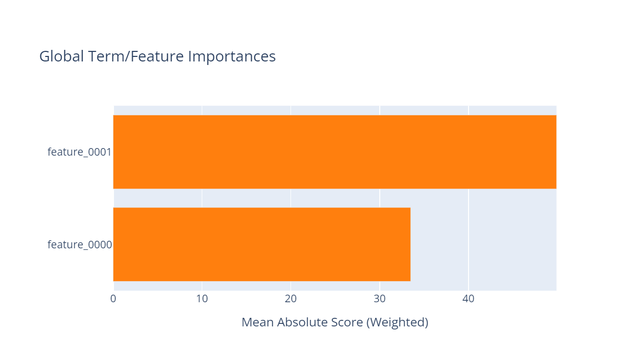
In this figure (taken from the official EBM documentation ⁷), you can see the feature names on the y-axis, and the mean absolute score of each feature (weighted) in the model on the x-axis. The scale of the y-axis is the same as the outcome scale. So one unit on the y-axis corresponds to one unit (increase or decrease, depending on the sign of course) of the outcome quantity that we predict.

The values are the averaged influence values of the respective features, computed on the training dataset. So we run our training dataset through the final model, sample by sample. And for each sample, we take its value for feature one and look up the associated predictive number for this feature. This number tells us, how the feature value contributes to the overall prediction. And we do this for every sample and for every feature in the training data, and then, simply average the results.

So the figure tells us, that the first features, on average, computed on the training data and given the model, increases the outcome (prediction) by 50 (whatever unit this is).

The second feature does the same but by 33.5.

So the first feature contributes much more to the prediction being a high, positive number than the second feature.

Local interpretability

Then we can look at the invidiual features, and see, which input value leads to which prediction for this feature. Using these values, we can explain the prediction of an individual sample (by just looking at the explainability of each feature value of the corresponding sample). The example is taken from the official EBM documentation ⁷

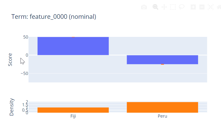
So this binary feature tells us, that having the categorical value for feature 1 of “Fijii” increases the outcome by a value of 50 while having a category of “Peru” decreases it by ~25.

Furthermore, we can find, at the bottom line of the graph, the Density of each value in the data (e.g. the histograms showing the relative number of occurrences of each of the possible values of the feature).

Classification Example (Binary and Multiclass) ^{8 9}

Global & Local interpretability

We are going to use the following example, for showing how to read the interpretability results of EBMs. The example uses the adult income dataset (https://archive.ics.uci.edu/ml/datasets/adult), and we use the features in the data to predict if the income is > 50k or <50k a year. So this example is for a classification task.

The figure axis is the same when comparing them to the regression case, but the scale is different. As in the binary case we map the model’s output to classes using a (inverse) logit function (as in logistic regression = classification), the scale here is on a log scale.

Why is that? To put it short: we actually are not only interested in how a feature influences the probability of a sample belonging to a certain class, but we are in fact interested in the probability of a sample belonging to a certain class - relative to the other class(es) in the data. We want to know, does this feature make the sample more likely to belong to class 0 or to class 1? And there is a concise way to put this intuition about interpretability in one single number: the concept of odds. The odds are a ratio that tells us exactly the answer to the previous question.

When $P(y_i=1)$ is our output probability that sample $i$ belongs to class 1, and $P(y_i=0)$ is the predicted probability that sample $i$ belongs to class 0 (in a two-class setting), then the odds are simply $\frac{P(y_i=1)}{P(y_i=0)}$ or with the laws of probability $\frac{P(y_i=1)}{1-P(y_i=1)}$. So the higher the odds, the more likely the event is to happen as opposed to it not happening. It is a good example of a contrastive explanation (and according to ¹ we humans love contrastive explanations).

So given this piece of information, how can we interpret these scores? Let’s lay the basis for doing so, by explaining the functions involved, that finally lead to the logarithmic odds we see on the y-axis of the interpretability plot.

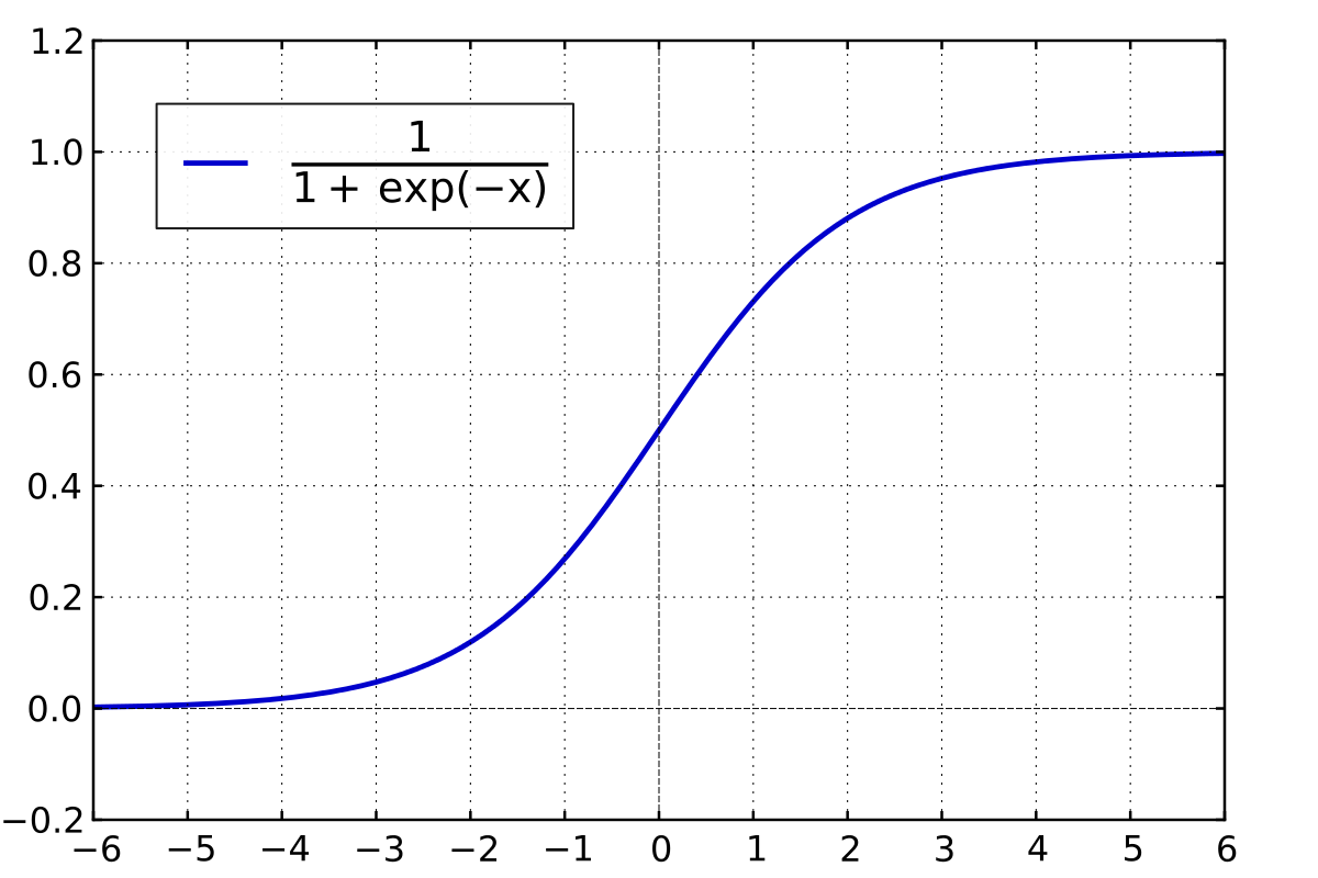
So the link function used is the logistic function, which maps the weighted sum of the model to a range of values between zero and one. Sounds like probabilities? That’s the idea behind it. In general, applying the logistic function on a plain linear regression model allows us to apply linear models to classification problems. The output domain is now restricted to be between zero and one and is no longer arbitrarily unbound. By then applying a threshold, let’s say a probability of 0.5, we can use the output of the logistic function to assign data points to one of two classes. The concept can be easily extended to n-classes, but for explaining the concept we will stick with the binary case.

Logistic function:

$\mathrm{logistic}(η)=\frac{1}{1+\mathrm{exp}^{-η}}$

That produces the following plot (for example, taken from wikipedia).

We will replace the parameter η with our regression EBM. As, in the end, we have one prediction per feature in our regression EBM, that are added together to get the final prediction, we will simply stick with these outputs to explain the effects of the logistic function on interpretability. For a single data point $x_i$ Let’s denote the overall output for feature $f$ of all $n$ features in our EBM model, by $y_{fi}$. So our final prediction $y_i$ for datapoint $i$ becomes, $\sum_{f\in n }{y_{fi}}$.

Why does the logistic function give us values between 0 and 1?

You can get a good sense of this when playing around with the values for η. If our prediction is very high, i.e., we have a high value for η, then we get a very large negative (due to the negotiation in the logistic function) number in the exponent of the denominator. $\mathrm{exp}$ to something very largely negative, converges to –> $lim_{x -> - \infin}\mathrm{exp}^x=0$. Thus, the larger our prediction gets the more we approach 1, as the all that remains in our logistic equation is $\frac{1}{1+0}=1$.

If we have very small predictions, we get close to zero, as $lim_{x -> + \infin}\mathrm{exp}^x=\infin$. Thus, our logistic equation becomes, roughly (not strictly mathematical for sure) $\frac{1}{1+\infin}=0$

So, we have values between zero and one now, despite orginally using our regression mode. Nice!

But the connection between the probabilities and our model predictions (and thus the feature relevance for each feature in our EBM) is not any longer linear (just look at the plot of the logistic function, does this look like a straight line to you :)? )

So what are these omninomous logits that are the are on the y-axis of your interpretation plot? Some terminiology (also checkout the wikipedia entry of logits on this matter).

An the log-odds, or short logits, are just the logarithm of the odds. So we have $ln\frac{p}{1-p}$. But we do not have probabilities yet. So the link function is not the logit function, but the inverse logisic function that we have described bevore.

Logistic function: Input to parameter η = our linear model (output) –> Output is a probability $P(y_i)$ for a class, e.g. $class=1$.

Logit (log-odds) function: Input is the probability for a class $P(y_i)$ and the output is the value for η = our linear model.

The interpretabilty function for the standard EBM is just doing this for us in the classification case. It take the class probabilities the EBM with the logistic link function has as an output, and turns them into logitc (log-odds) for getting the connecting of the probability output to the model parameters again.

So the logits give us the following relationship, given the EBM result $P(y_i)$ for sample $i$.

$ln(\frac{P(y_i)}{1-P(y_i)})= η = \mathrm{our \space EBM \space model} = \sum_{f\in n }{y_{fi}}$

So to check what the influece of an increase of the prediction output $y_{fi}$ of feature $f$ for sample $i$ has on the overall probability $P(y_i=1)$ of sample $i$ getting classified as class $1$, we can check what happens with the ratio of our EBM output. So we just take the prediction value $y_{fi}$ as it is by our trained EBM, and we use one fictive EBM with our prediction value $y_{fi}$ increased by one, thus $y_{fi}+1$.

Using the logit (log-odds) function, we can compare the probabilities by comparing the log-odds of the “real” and the “fictive” (+1 unit) EBM outputs.

Thus, when aiming to relate changes in the features to probabilities of belonging to a class, we can look at the relative logits for this feature. So if we have logits (log-odds) of two for example, this means that the probability for $P(y_i)$ is twice as high as the probability for $1-P(y_i)$ (the counter event), when there is a one unit increase in feature $y_{fi}$.

Relationship between log-odds (logit) and logistic function As they are inverse, applying both functions to an input results in the identity function (i.e. nothing happens with the input). Check out this link for the mathematical derivation, it is quite straight forward with a tiny trick involved to make the equations easier (do not worry, this tricks is pulled of from “nowhere” … at least it looks like that. but have a closer look at the equations when introducing the multiplication by “1”)

Wrapping this up for Classification:

Logit Scale y-axis means: this is the influece of each feature on the logit, i.e. on the logarithmic odds of an event happening vs. it not happening. (of a sample belonging to class 1 vs. it belonging to class 0).

If you want to get the actual influence of a unit increase of a numerical feature i by 1 on the output, you can apply $\mathrm{exp}$ to the feature value to get its influece on the odds of the event happeing vs. it not happening. You get rid of the “logarithm” part of the log-odds by doing so ¹.

For a binary categorical variable, changing from the reference category to the other category, leads to an influence on the log odds of $\mathrm{exp}(\mathrm{value})$ too. For multi-category features it depends on the category encoding of the feature in the model. In case of one-hot encoding, we have plenty of binary ones again :) Makes stuff easier.

To conclude …

EBMs are one of my favourite tools for solving real world problems for clients that want to have high predictive accuracy and high interpretability. And in fact, this is the standard set of requirements :) Thanks for developing this kind of model dear Microsoft Research!

---

Other sources on EBMs include ^{3 7 8 9 10 11 2 6 12 13 4 5}

1. Book “Interpretable Machine Learning: A guide for making black box models interpretable” by Christoph Molnar. ↩ ↩² ↩³

2. Paper: Intelliiglbe models for classification and regression https://www.cs.cornell.edu/~yinlou/papers/lou-kdd12.pdf ↩ ↩² ↩³ ↩⁴ ↩⁵ ↩⁶ ↩⁷ ↩⁸

3. EBM general: https://interpret.ml/docs/ebm.html ↩ ↩² ↩³ ↩⁴

4. Gradient Boosting Wikipedia: https://en.wikipedia.org/wiki/Gradient_boosting#:~:text=Gradient%20boosting%20is%20a%20machine,which%20are%20typically%20decision%20trees ↩ ↩² ↩³ ↩⁴

5. EBM youtube: https://www.youtube.com/watch?v=MREiHgHgl0k ↩ ↩²

6. Paper: Accurate intelligible models with pairwise interactions” (Y. Lou, R. Caruana, J. Gehrke, and G. Hooker 2013) https://www.cs.cornell.edu/~yinlou/papers/lou-kdd13.pdf ↩ ↩²

7. EBM regression: https://interpret.ml/docs/ebm-internals-regression.html ↩ ↩² ↩³ ↩⁴

8. EBM binary classification: https://interpret.ml/docs/ebm-internals-classification.html ↩ ↩²

9. EBM multi-class classification: https://interpret.ml/docs/ebm-internals-multiclass.html ↩ ↩²

10. EBM blogpost: https://towardsdatascience.com/ebm-bridging-the-gap-between-ml-and-explainability-9c58953deb33 ↩

11. InterpretML Paper: https://arxiv.org/abs/1909.09223 ↩

12. Paper: “Interpretability, Then What? Editing Machine Learning Models to Reflect Human Knowledge and Values” (Zijie J. Wang, Alex Kale, Harsha Nori, Peter Stella, Mark E. Nunnally, Duen Horng Chau, Mihaela Vorvoreanu, Jennifer Wortman Vaughan, Rich Caruana 2022) ↩

13. Gradient Boosting Blog: https://towardsdatascience.com/all-you-need-to-know-about-gradient-boosting-algorithm-part-1-regression-2520a34a502 ↩